12 F-h analysis
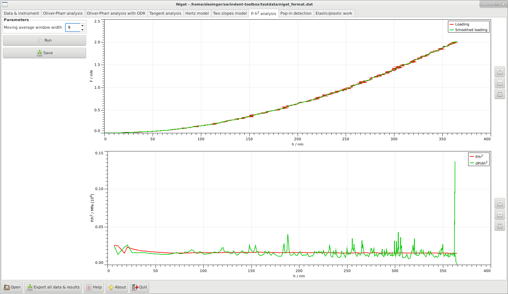
12.1 Window
The window consists of several blocks:
-
•
Parameters allows the user to set the width of the moving average window. The value 1 corresponds to no smoothing. This value is saved in settings.
-
•
Run perform calculation and display curve, see section 12.2.
-
•
Save save parameters and results to given file.
-
•
Graph
-
Top: display the loading curve and the smoothed curve.
-
Bottom: display the
 and the
  curves.
Stepwise zooming/unzooming can be performed by selecting a range with the mouse and pressing the Zoom/ Unzoom buttons. The graph is restored to its original size by the Restore button. Zooming in the two graphs is independent.
-
12.2 Procedure
-
1.
We use a moving average with a fixed width and constant weight. This means we substitute a value with its average with
 values to the left and to the right,
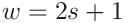
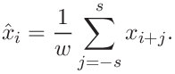
The value
 corresponds to the original data. There is only one moving average type defined for both depth and load.
Increasing the value of
corresponds to the original data. There is only one moving average type defined for both depth and load.
Increasing the value of  noise becomes less influential but important small effects can get lost as well.
Therefore, the value should not be too large, below 11 is recommended.
noise becomes less influential but important small effects can get lost as well.
Therefore, the value should not be too large, below 11 is recommended. -
2.
The ratio
is calculated for for each data pair  of the (smoothed) loading curve and plotted as a function of the (smoothed) depth
  .
. -
3.
The derivative
is calculated for for each data pair of the (smoothed) loading curve and plotted as a function of the (smoothed) depth .
The derivative is done numerically as the ratio of the derivatives of  and
and  with respect to the (time)step or index
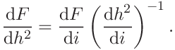
The numerical derivatives are calculated using the three-point formula for equally spaced data.
![[LOGO]](data:image/png;base64,iVBORw0KGgoAAAANSUhEUgAAAAsAAAAOCAYAAAD5YeaVAAAAAXNSR0IArs4c6QAAAAZiS0dEAP8A/wD/oL2nkwAAAAlwSFlzAAALEwAACxMBAJqcGAAAAAd0SU1FB9wKExQZLWTEaOUAAAAddEVYdENvbW1lbnQAQ3JlYXRlZCB3aXRoIFRoZSBHSU1Q72QlbgAAAdpJREFUKM9tkL+L2nAARz9fPZNCKFapUn8kyI0e4iRHSR1Kb8ng0lJw6FYHFwv2LwhOpcWxTjeUunYqOmqd6hEoRDhtDWdA8ApRYsSUCDHNt5ul13vz4w0vWCgUnnEc975arX6ORqN3VqtVZbfbTQC4uEHANM3jSqXymFI6yWazP2KxWAXAL9zCUa1Wy2tXVxheKA9YNoR8Pt+aTqe4FVVVvz05O6MBhqUIBGk8Hn8HAOVy+T+XLJfLS4ZhTiRJgqIoVBRFIoric47jPnmeB1mW/9rr9ZpSSn3Lsmir1fJZlqWlUonKsvwWwD8ymc/nXwVBeLjf7xEKhdBut9Hr9WgmkyGEkJwsy5eHG5vN5g0AKIoCAEgkEkin0wQAfN9/cXPdheu6P33fBwB4ngcAcByHJpPJl+fn54mD3Gg0NrquXxeLRQAAwzAYj8cwTZPwPH9/sVg8PXweDAauqqr2cDjEer1GJBLBZDJBs9mE4zjwfZ85lAGg2+06hmGgXq+j3+/DsixYlgVN03a9Xu8jgCNCyIegIAgx13Vfd7vdu+FweG8YRkjXdWy329+dTgeSJD3ieZ7RNO0VAXAPwDEAO5VKndi2fWrb9jWl9Esul6PZbDY9Go1OZ7PZ9z/lyuD3OozU2wAAAABJRU5ErkJggg==)