15 Uncertainties
Uncertainties can be calculated for the Oliver Pharr method (either fitting procedure), the tangent method and the Hertz method.
The uncertainty sources are the noise in the depth and load, the uncertainty in the tip radius (Hertz method) and the uncertainties in the material parameters (Poisson’s ratio, Young’s modulus and Poisson’s ratio of indenter).
These are treated by the Gaussian propagation of uncertainties. The Monte Carlo method is used to treat the noise of depth load. In all cases we use a normal distribution and assume zero correlation (also between different depth values, i.e. ![]() ).
The uncertainty of the contact point is demonstrated separately by explicitly performing the evaluation of data with different contact points and comparing them.
The uncertainty of the choice of the fitting interval is not implemented yet.
).
The uncertainty of the contact point is demonstrated separately by explicitly performing the evaluation of data with different contact points and comparing them.
The uncertainty of the choice of the fitting interval is not implemented yet.
15.1 Window
In all cases, pressing the Uncertainties button opens a separate window with the following blocks
-
•
Uncertainties in input values the user can calculate the uncertainties and the individual contributions to the contact depth and area, indentation hardness and modulus and contact modulus. For the Hertz method only the uncertainties of the contact and indentation modulus are available. These contributions are calculated using the propagation of uncertainties [7]. Details are in sections 15.2.1, 15.2.2, 15.2.4.
-
•
Uncertainties due to choice of contact point shows results, that would be obtained, if the contact point had been chosen differently. In many cases it is non-trivial how to choose the contact point, so this can be a significant contribution to the overall uncertainty.
-
•
Save Save the resuls of the uncertainty analysis, including the main results of the corresponding main calculation, as the uncertainty analysis refers only to this calculation.
-
•
Monte Carlo calculation of uncertainties set the number of iterations and launch the calculation of the uncertainties using the Monte Carlo method [6, 5]. In [6, 5] a minimum value of 10 000 is recommended, however, results obtained with smaller values can be used with proper care as a first guess. For ODR, one should start with approx. 100, and then gradually increase, as this is significantly more time consuming. The procedure is described in section 15.4.
Only one Uncertainty window may be open for each method. Values of uncertainties are saved in (and loaded from) the settings file for future use.
15.2 Gaussian propagation of uncertainties
The standard treatment to uncertainties is described in [7]. Here we use only the most important results.
Let two quantities ![]() and
and ![]() be estimated by
be estimated by ![]() and
and ![]() and depend on a set of uncorrelated variables
and depend on a set of uncorrelated variables ![]() .
Let
.
Let ![]() be the estimated variance of the estimate
be the estimated variance of the estimate ![]() of
of ![]() .
Then the estimated variance associated with
.
Then the estimated variance associated with ![]() is given by
is given by
 |
(30) |
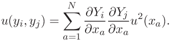
and the estimated covariance associated with ![]() and
and ![]() is given by
is given by
 |
(31) |
Let ![]() be estimated by
be estimated by ![]() and depend on the correlated quantities
and depend on the correlated quantities ![]() . Let
. Let ![]() be the estimated variance of the estimate
be the estimated variance of the estimate ![]() of
of ![]() and
and ![]() the estimate of the covariance associated with
the estimate of the covariance associated with ![]() and
and ![]() for
for ![]() .
Then the estimated variance associated with
.
Then the estimated variance associated with ![]() is
is
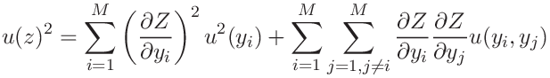 |
(32) |
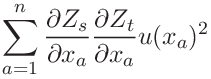
The covariance of variables ![]() depending on the independent random variables
depending on the independent random variables ![]() through intermediate variablse
through intermediate variablse ![]() can be computed as.
can be computed as.
 |
(33) | ||||
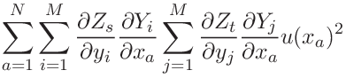 |
(34) | ||||
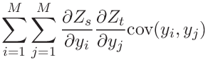 |
(35) |
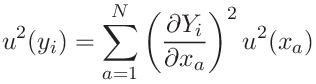
In our case the independent variables ![]() are the depth values
are the depth values ![]() , load values
, load values ![]() . We assume that they are all have a normal distribution function with the same variance, i.e.
. We assume that they are all have a normal distribution function with the same variance, i.e.
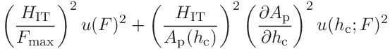
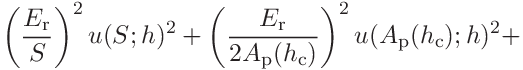
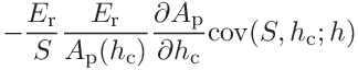
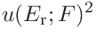
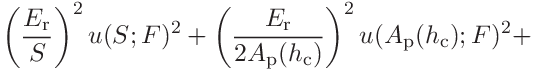
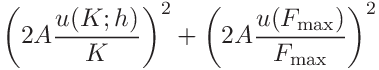
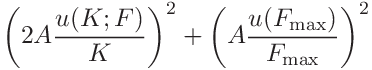
Equation (30) can then be written as the sum of two terms: the sum of the contributions from the depth data and from the force data
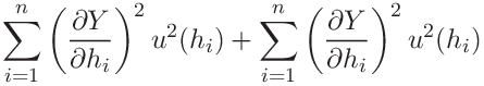 |
||||
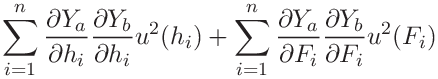 |
||||
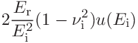
For the indentation modulus we additionally need the tip radius ![]() , Poisson’s ratio
, Poisson’s ratio ![]() , Young’s modulus of the indenter
, Young’s modulus of the indenter ![]() and Poisson’s value of the indenter
and Poisson’s value of the indenter ![]() . We assume that they are independent and have a normal distribution.
. We assume that they are independent and have a normal distribution.
15.2.1 Uncertainty propagation for Oliver Pharr method with ODR
The package ODRPACK does not allow to separate the contributions from depth and load uncertainty. The results which correspond to a fit using only the uncertainties in the depth, resp. load are shown instead of the contributions and the result from a fit using both uncertainties is shown instead of the combined uncertainty.
-
1.
Obtain the uncertainties of
 and
and  , as well as their covariance from ODRPACK, see A.1.
 -
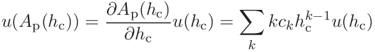
2.
Calculate the uncertainty of
 from equation (6).
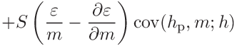
For we find

![\displaystyle u(m;h)\left[\frac{\varepsilon}{m}-\frac{\varepsilon-m}{m-1}-%
\frac{\varepsilon-m}{2(m-1)^{2}}(\psi_{0}(z)-\psi_{0}(w))\right],](mi/mi266.png)
(36) with
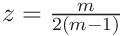 , and
, and 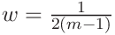 and similarly for
  .
The derivative
.
The derivative  is needed in further calculations
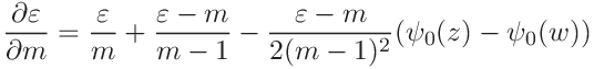
(37) -
3.
For
 we get

For
 we obtain

(39) 
(40) 
- 4.
-
5.
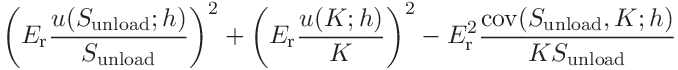
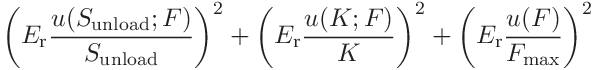
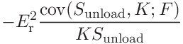
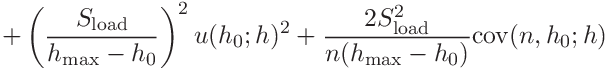
The two contributions to the hardness are
(42) 
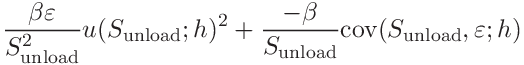
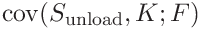
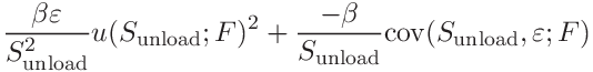
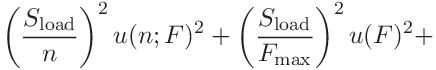
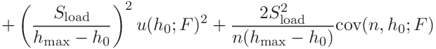
The two contributions to the contact modulus are
(44) 
(45) 
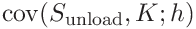
where the covariances
 and
and  are
are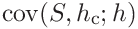
(46) 
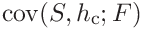
(47) 
-
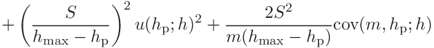
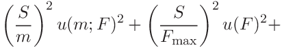
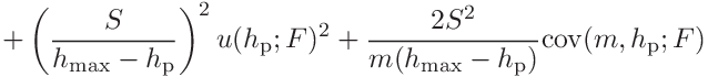
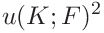
6.
Combine the uncertainties originating in depth and load
 and
and  with the uncertainties of the material parameters
  ,
,  and
and  .
The contributions are
.
The contributions are
(48) 
(49) 
(50) 
(51)
15.2.2 Uncertainty propagation for Hertz method with ODR
- 1.
-
2.
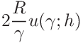
If the tip radius was given, the contributions to the uncertainty of the contact modulus are


- 3.
-
4.
If the contact modulus was given the contributions to the uncertainty of the radius are


-
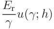
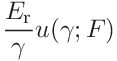
5.
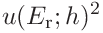
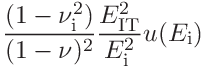
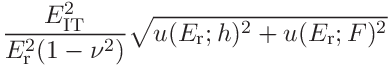
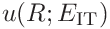
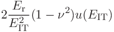
If the indentation modulus was given the uncertainties can be expressed in terms of the contact modulus
![E_{\mathrm{r}}=\left[\frac{1-\nu^{2}}{E_{\mathrm{IT}}}+\frac{1-\nu_{\mathrm{i}%
}^{2}}{E_{\mathrm{i}}}\right]^{-1}](mi/mi145.png)
as


15.2.3 Uncertainty propagation for stiffness analysis
The package ODRPACK does not allow to separate the contributions from depth and load uncertainty.
The results which correspond to a fit using only the uncertainties in the depth, resp. load are shown instead of the contributions and
the result from a fit using both uncertainties is shown instead of the combined uncertainty.
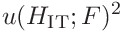
The uncertainties of ![]() ,
, ![]() ,
, ![]() and
and ![]() are obtained directly from ODRPACK, see A.1
are obtained directly from ODRPACK, see A.1
15.2.4 Uncertainty propagation for two slopes method with ODR
The package ODRPACK does not allow to separate the contributions from depth and load uncertainty.
The results which correspond to a fit using only the uncertainties in the depth, resp. load are shown instead of the contributions and
the result from a fit using both uncertainties is shown instead of the combined uncertainty.
In the following we assume that neither fit includes the ![]() point and that the fits are independent.
point and that the fits are independent.
-
1.
Obtain the uncertainties of
 ,
,  , , , and their covariance from ODRPACK, see A.1.
 - 2.
- 3.
-
4.
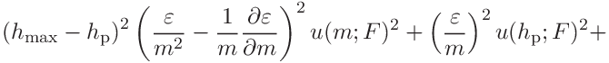
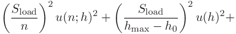
It is practical to calculate the uncertainties of the auxiliary term
 given as
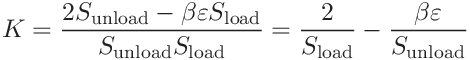
(54) These are


We will also need the covariance
-
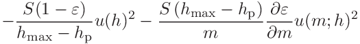
5.
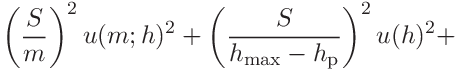
In terms of
the uncertainties of the contact area, hardness and contact modulus can be expressed as
and
(59) 
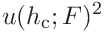
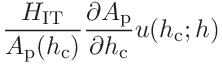
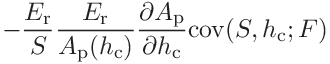
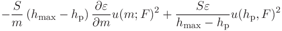
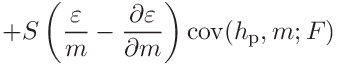
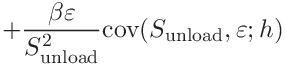
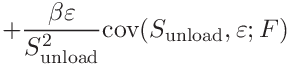
- 6.

![\displaystyle\frac{\partial\varepsilon}{\partial m}\left[m\frac{F_{\mathrm{max%
}}}{(h_{\mathrm{max}}-h_{\mathrm{p}})^{2}}\mathrm{cov}(h_{\mathrm{p}},m;h)+%
\frac{F_{\mathrm{max}}}{h_{\mathrm{max}}-h_{\mathrm{p}}}u(m;h)^{2}\right]](mi/mi159.png)
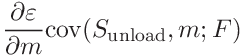
![\displaystyle\frac{\partial\varepsilon}{\partial m}\left[m\frac{F_{\mathrm{max%
}}}{(h_{\mathrm{max}}-h_{\mathrm{p}})^{2}}\mathrm{cov}(h_{\mathrm{p}},m;F)+%
\frac{F_{\mathrm{max}}}{h_{\mathrm{max}}-h_{\mathrm{p}}}u(m;F)^{2}\right]](mi/mi158.png)
15.3 Uncertainty due to choice of contact point
It may not be always clear where exactly the contact between the indenter and the sample occurs. This induces an uncertainty of type B which must be estimated.
In order to facilitate this, we explicitly show how the results change when the contact point was chosen to be more to the left or to the right by a certain amount of points.
Zero contact point shift means the original contact point was used. A positive (negative) contact point ![]() shift means the
shift means the ![]() th neighboring point to the right (left) was used instead.
This corresponds to a shift by
th neighboring point to the right (left) was used instead.
This corresponds to a shift by ![]() in the unloading data; data are added or removed from the loading data as well as shifted by
in the unloading data; data are added or removed from the loading data as well as shifted by ![]() .
The ranges for the interval of the fitting procedures are transformed. If they were chosen in the length regime, either by mouse or by input in the entries, they are shifted by
.
The ranges for the interval of the fitting procedures are transformed. If they were chosen in the length regime, either by mouse or by input in the entries, they are shifted by ![]() .
Percentages of the maximum forces are not transformed, since the maximum force is already shifted.
.
Percentages of the maximum forces are not transformed, since the maximum force is already shifted.
15.4 Monte Carlo calculation of uncertainties
The calculation is run by clicking the Monte Carlo button in the Uncertainty window. After finishing a window containg the results is shown. The calculation itself is described in 15.4.2. A more detailed description of the use of the Monte Carlo method for the evaluation of uncertainties is in [6, 5].
15.4.1 Window
-
•
Input of Monte Carlo simulation shows the input values with which the calculation was run.
-
•
Results of Monte Carlo simulation shows the mean and standard deviation calculated from the resulting PDFs. A histogram can be shown by clicking on the histogram button for each variable.
-
•
Save save the results of this Monte Carlo simulation. This includes the mean, standard deviation, histogram and full data for each output variable.
Only one Monte Carlo calculation window may be open for each method. It is closed when the Uncertainty window is closed and results are discarded.
15.4.2 Monte Carlo calculation of uncertainties: Description of method
A more detailed description of the use of the Monte Carlo method for the evaluation of uncertainties is in [6, 5]. The procedure is based on the propagation of probability distribution functions (PDF) of the input variables and obtaining the PDF of the output variable. The input variables are varied according to a given PDF and the output variables are calculated in each case. For a large enough number of trials we obtain a PDF of the output variables, which can be further analyzed. Here we calculate only the mean and the standard deviation and construct a simple histogram. This method is very well suited for complicated measurement models, especially non-linear models or non-Gaussian PDFs of the input variables. In simple cases, it gives the same results as the Gaussian law of propagation. Two Monte Carlo method has two significant drawbacks compared to the Gaussian law of propagation: Firstly, it can become very time consuming, especially when several input variables are present. Secondly, it is impossible to separate the uncertainty contributions from different input variables. Different calculations must be made, thus increasing even more the time needed. Therefore, it is currently used only for the uncertainty in the depth and the load. The uncertainties in the material parameters and the tip radius (Hertz model) can be described sufficiently by the Gaussian law. The model uses independent, normal PDFs with constant variance for all depth and load values. Only values contained in the fitting range of the main calculation are considered, i.e., the fitting range is not determined for every individual calculation. This leads to a significant speed up. For well-behaved data, this should not cause any significant errors.
![[LOGO]](data:image/png;base64,iVBORw0KGgoAAAANSUhEUgAAAAsAAAAOCAYAAAD5YeaVAAAAAXNSR0IArs4c6QAAAAZiS0dEAP8A/wD/oL2nkwAAAAlwSFlzAAALEwAACxMBAJqcGAAAAAd0SU1FB9wKExQZLWTEaOUAAAAddEVYdENvbW1lbnQAQ3JlYXRlZCB3aXRoIFRoZSBHSU1Q72QlbgAAAdpJREFUKM9tkL+L2nAARz9fPZNCKFapUn8kyI0e4iRHSR1Kb8ng0lJw6FYHFwv2LwhOpcWxTjeUunYqOmqd6hEoRDhtDWdA8ApRYsSUCDHNt5ul13vz4w0vWCgUnnEc975arX6ORqN3VqtVZbfbTQC4uEHANM3jSqXymFI6yWazP2KxWAXAL9zCUa1Wy2tXVxheKA9YNoR8Pt+aTqe4FVVVvz05O6MBhqUIBGk8Hn8HAOVy+T+XLJfLS4ZhTiRJgqIoVBRFIoric47jPnmeB1mW/9rr9ZpSSn3Lsmir1fJZlqWlUonKsvwWwD8ymc/nXwVBeLjf7xEKhdBut9Hr9WgmkyGEkJwsy5eHG5vN5g0AKIoCAEgkEkin0wQAfN9/cXPdheu6P33fBwB4ngcAcByHJpPJl+fn54mD3Gg0NrquXxeLRQAAwzAYj8cwTZPwPH9/sVg8PXweDAauqqr2cDjEer1GJBLBZDJBs9mE4zjwfZ85lAGg2+06hmGgXq+j3+/DsixYlgVN03a9Xu8jgCNCyIegIAgx13Vfd7vdu+FweG8YRkjXdWy329+dTgeSJD3ieZ7RNO0VAXAPwDEAO5VKndi2fWrb9jWl9Esul6PZbDY9Go1OZ7PZ9z/lyuD3OozU2wAAAABJRU5ErkJggg==)